

Software manual
ChipScan-Scanner 3.0
Notice! No part of this manual may be reproduced in any form or by any means (including electronic storage and retrieval or translation into a foreign language) without prior agreement and written consent from Langer EMV-Technik GmbH. The management of Langer EMV-Technik GmbH assumes no liability for damages which may result from the use of this printed information.
Overview
ChipScan-Scanner is an evaluation software designed for reliable acquisition, fast inter-active visualization and sophisticated analysis of electromagnetic compatibility (EMC) measurements of components. In combination with a Langer IC-Scanner and one of Langer's ICR microprobes, ChipScan-Scanner is a versatile tool for measuring high-frequency magnetic or electric fields up to 6 GHz of integrated circuits, PCBs and evencomplete products.
ChipScan-Scanner key features
- Reliable configuration and measurement of emission scans
ChipScan-Scanner allows the quick configuration and reliable execution of surface emission scans using one of Langer's IC-Scanners. Additional to common surface scans ChipScan-Scanner supports scanning a specific volume over a DUT. So not only you gather information of the electric and magnetic fields at the DUT's surface but you gain information about the 3D distribution of the fields in the proximity of the DUT, too.
All settings of a scan including the used spectrum analyzer1 are automatically stored in a protocol for later use. Thus future measurements with identical properties are achieved easily without any fault. - Fast visualization of scans for evaluation of near field emissions
Depending on scan type, ChipScan-Scanner enables you to visualize and manipulate up to 300,000 measurement points in real-time, which is essential for high-resolution EMC scans. Furthermore, ChipScan-Scanner is not limited to create a surface or volume plot for specific frequencies. You can also generate plots containing the maxima of the field intensities for freely definable frequency bands. As well you can visualize isosurfaces of the field intensities. Thus DUT's interference processes can be systematically understood and thoroughly analyzed. - Sophisticated processing of emission scans
ChipScan-Scanner provides some important processing features to make an exact and detailed analysis of near field emissions even easier. You can subtract a reference measurement of your DUT from any subsequent scan of the very same or a different DUT. So locating and documenting the outcome of changes in a devices' design process can be achieved very quickly. This method is very useful to automatically verify near field emissions throughout your production, too.
Furthermore the traces of all measurement points can be compared to each other or can be compared with traces of other measurements which allows a detailed frequency based analysis of the near field. - Image and data export for documentation, statistical analysis, etc.
All rendered images can be easily exported in various image formats. Thus you can easily generate any needed documentation or presentation of your work regarding a specific EMC problem. Additionally ChipScan-Scanner can export all traces of a specific emission scan to a comma separated value list (.csv) for futher statistical analysis with tools like R, Matlab or Excel. - Reliable storage of emission scans for future usage
You can store all scans to continue your evaluation at a later stage, allowing an evaluation independent from the measurement of an emission scan. This can be especially useful for specific protocols when different people are responsible for acquisition and evaluation.
Support
Our software team provides uncomplicated support in case of problems, questions or requests concerning ChipScan-Scanner. Please contact us by writing to software@langer-emv.de. You may check our website http://www.langer-emv.com/ from time to time for new releases of ChipScan-Scanner, too.
If you have any feature or custom development request that should be implemented immediately please contact our sales team using the following email address mail@langer-emv.com.
1.System requirements and installation
1.1. System requirements
Your computer system should have at least the following properties.
- 1 GB HD space
- CD drive for installation of ChipScan-Scanner
- Windows ®7 64-bit (latest service packs)
- Monitor with a display resolution of 1280x1024 or greater
- Spectrum analyzer1 (for trace acquisition only)
The minimum memory requirements strongly depend on the number and the size of the loaded emission scans, whereas the minimum CPU and GPU requirements strongly depend on the size of the displayed emission scan. Because of these circumstances we just provide a recommended setup for RAM, CPU and GPU. This setup is able to load at least three emission scans each consisting of 100,000 measurement points2, and to visualize and to manipulate them in real-time.
Because of these circumstances we just provide a recommended setup for RAM, CPU and GPU. This setup is able to load 10,000 traces each having 1,000 data points and to display about 1,000 of them without any latency.
- 2 GB of RAM
- CPU Intel Core i7 2.7 GHz
- GPU AMD Radeon 7950 with 3 GB of GDDR5 memory
1.2. Installation
- Insert the ChipScan-Scanner CD into your CD-ROM drive.
- Change to the directory ChipScan-Scanner on the CD.
- Double click ChipScan Scanner.exe
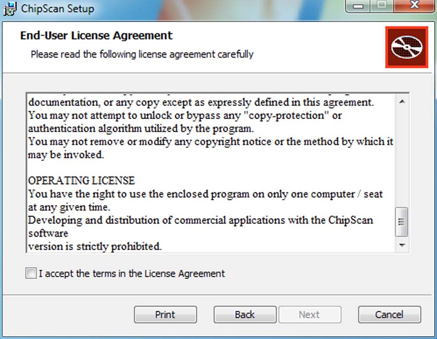
- Please read the license agreement carefully. If you accept it, you can go on.
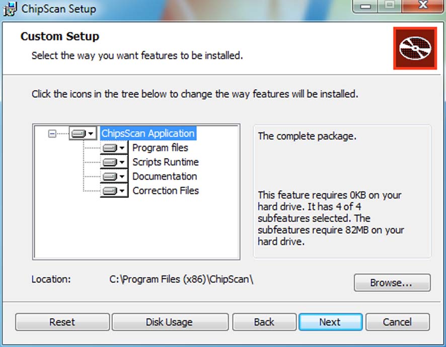
- Select the location where ChipScan-Scanner will be installed.
- Finish installation.
1.3. Start
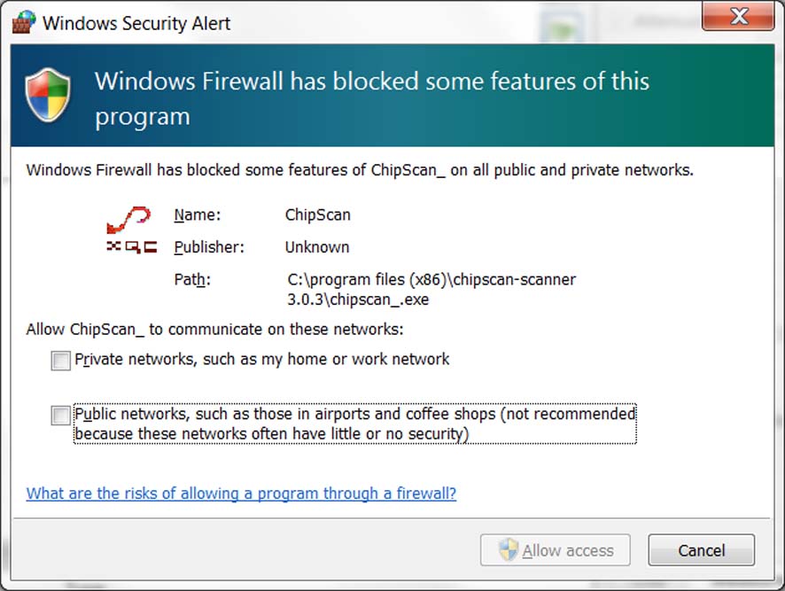
At ChipScan-Scanner first start a Windows Security Alert dialog may appear (see Figure 1.1). This is due to the integrated XMLRPC server, see section 6 for details. Choose the Cancel button to close this dialog.
2. Getting Started
2.1. Quick introduction into ChipScan-Scanner
For users who want to get started immediately here is a quick introduction to ChipScan-Scanner. The example data files used in this tutorial can be found in the data directory in your ChipScan-Scanner distribution or can be downloaded from our website http://www.langer-emv.com/chipscan
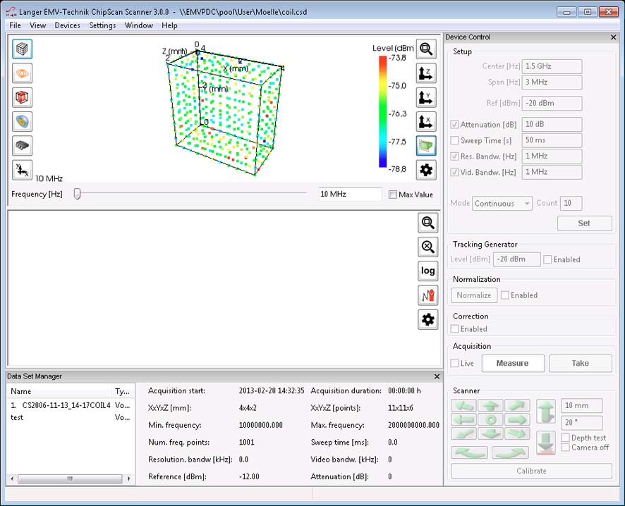
Start ChipScan-Scanner by clicking the ChipScan icon on your desktop or in the Application menu. ChipScan-Scanner will start up with the main window entitled ChipScan-Scanner (see Figure 2.1).
The main window allows the viewing of six different dock windows: the visualization which is always visible, the data set manager, the device control, the trace manager, the scan manager and the log. If you closed any of these windows you can make them visible by selecting the appropriate menu item in the Window menu.
2.2. Viewing of surface and volume emission scans
To open an emission scan file select Open... in the File menu. Navigate in the file dialog to the directory where the example data files are located and mark the desired file with a single (left) mouse click. Pressing the Open button opens the file. With the default dock window settings you see the visualization in the center displaying the emission scan, the device control on the right next to it and the data set manager on the bottom (see Figure 2.1). In the following we only present a small overview of the visualization features, see section 3.2 for further details.
In the upper part of the visualization all measurement points of the emission scan are shown for a specific frequency within the acquired frequency range. Each point has a specific color that maps to a corresponding value in the color bar on the right. Adding or removing any additional information like isosurfaces or an image of your DUT can be achieved via the buttons on the left next to the visualization. Use the slider on thebottom of the visualization to switch between frequencies and display the appropriate information.
In addition to viewing specific information of your emission scan you can navigate within the scan, too. To rotate the emission scan in any direction around the center of the scene move the mouse over the visualization while holding down the left mouse key. You may additionally hold down the Ctrl key to rotate the scan around the projection axis only. Holding down the Shift key instead will move the scan along the projectionplane. You can zoom in/out of the scan by spinning the scroll wheel. When moving the mouse pointer over a specific measurement point of the emission scan you will see the specific trace of this point in a Cartesian coordinate system below.
Furthermore you can adjust several properties of the emission scan visualization to satisfy your specific needs. For example you can change the transparency of the isocontours or set the position and size of the DUT image in the scene. To do this press the  button on the right next to the scan visualization. In the subsequent dialog all properties are grouped into different categories and therefore can be easily found and altered.
2.3. Single trace analysis
As was pointed out in section 2.2, you can view the trace of any measurement point in the lower part of the visualization, by moving the mouse pointer over it. To add any trace permanently do a right mouse click on the appropriate measurement point and select Add To Trace Visualization from the subsequent context menu. In this way you can easily compare the trace of any points of the emission scan against one another and even against a separate reference.
To better keep track of different traces within the visualization you can manage a trace's properties like visibility and color via the trace manager. To open it press Ctrl+T or select the Trace Manager entry from the Window menu.
In addition you have multiple navigation options in the trace visualization to analyze specific trace frequencies in detail. You can center a point of interest in the traces by moving the mouse while holding down the left mouse key over the visualization. You can zoom in/out of the traces by spinning the scroll wheel. While spinning you may also hold down the Shift or the Ctrl key to zoom along the x- or y-axis only. Moving themouse pointer over a data point of a trace will display the specific values for x/y-axis including the unit. To recover the full view range of all visible traces press the  button on the right next to the trace visualization.
2.4. Acquiring single traces and emission scans
To acquire emission scans using ChipScan-Scanner it is required that you connect a spectrum analyzer1 and one of Langer's IC-Scanners to your PC. Make sure both devices are properly connected. Furthermore, to eliminate any connection problems regarding your spectrum analyzer you may verify your setup with a software provided by the spectrum analyzer manufacturer.
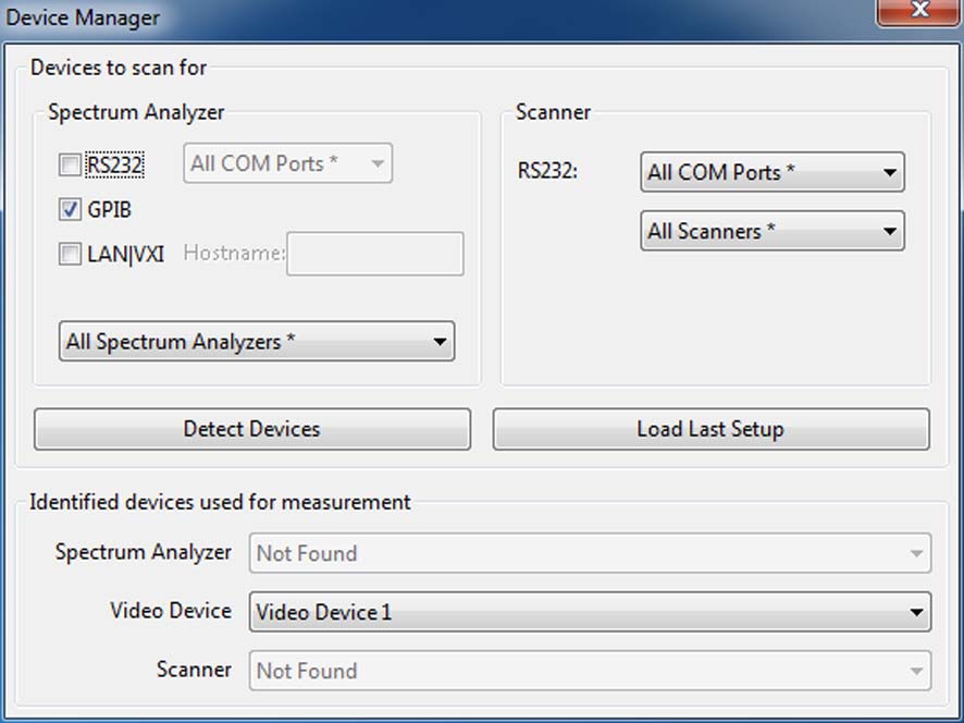
Before starting the data acquisition you must detect both the spectrum analyzer and the Langer's IC-Scanner that are connected to your PC. To do so select Device Manager from the Devices menu. In the subsequent device manager dialog (see Figure 2.2) select the interface your spectrum analyzer is connected to and press the Detect Devices button. All connected devices, which have been automatically identified, willbe shown in the Identified devices used for measurement section of the dialog. Make sure to select your connected spectrum analyzer from the list of identified devices. If your spectrum analyzer could not be automatically identified please redo the afore mentioned connection test. If it does not succeed please see section 4 for a detailed description of the device manager and its capabilities before contacting our support.
2.4.1. Single traces
After identifying the connected spectrum analyzer you can change all important properties like frequency range, reference level, etc. of the spectrum analyzer via the device control (see Figure 2.1). To finally set the properties press the Set button. This will transferall settings to the spectrum analyzer. If your spectrum analyzer includes a supported tracking generator you may configure it, too. When finished you can acquire a trace by pressing the Measure or Take button. The trace will be shown in the visualization. The visibility and other properties of any single trace can be altered via the trace manager.
2.4.2. Emission scans
 | Attention: Any of the following steps for scanner control may cause damage to any equipment and serious injuries or death to persons within the motion range of the scanner. Please proceed with caution while keeping all safety measures. |
Before you start to work with the identified IC-Scanner you must initiate a calibration routine by pressing the Calibrate button in the scanner section of the device control. This will initialize the scanner and move all axes to their zero-point position. Afterwards the ICR microprobe can be moved and rotated by setting the motion distance and rotation angle, and pressing the arrow buttons. If the probe is finally positioned at thestart point of your measurement you need to activate the scan manager to acquire an emission scan.
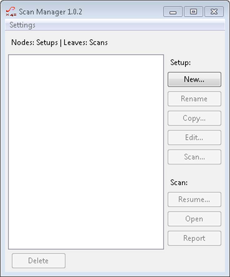
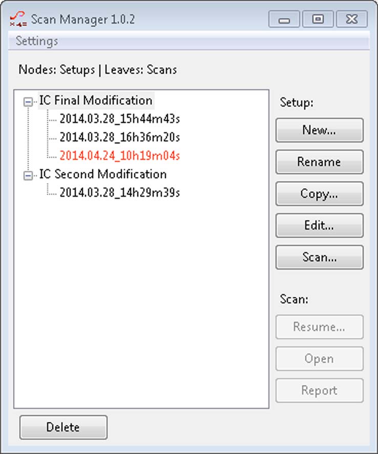
To activate the scan manager select the Scan Manager entry from the Window menu. In the scan manager (see Figure 2.3) you need to create a new scan setup by pressing the New button. After naming the scan setup in the subsequent dialog you are presented with a configuration dialog for the setup. Among other settings you can specify the dimensions of the volume you want to scan. You can leave the preset settings3 and press the Ok button of the dialog to return to the scan manager.
After the new scan setup is created you need to press the Scan button in the scan manager. This will initialize the visualization of ChipScan-Scanner and in the subsequent dialog you can start the scan. During the execution of the scan the dialog shows the remaining time amongst other things and the visualization of ChipScan-Scanner is updated, too.
After the scan is finished you may view the appropriate report by pressing the Report button in the scan manager. To further analyze your emission scan data close the scan manager and follow the description in section 2.2.
2.5. Exporting data and images
Beside saving of acquired emission scans you can also export all of one's traces. This is especially important for further analysis with statistical software like R or Matlab. To do so select Export data... from the File menu and specify the file in the subsequent file dialog where the data should be saved to. The resulting file (.csv) will contain a comma separated value list of all traces currently available in the data manager.
Furthermore you may want to export the image of the current visualization for purposes like presentation or documentation. To do so select Export Scan Image... or Export Traces Image... from the File menu and a file dialog will open. There select a filename and an image type to finally save the image in a file.
3. Graphical user interface
The layout of the graphical user interface of ChipScan-Scanner is partly configurable to meet your demands during different tasks. It uses a dock window system, which allows to rearrange some windows of the graphical user interface within the main window. Apart from the visualization there are three main dock windows, the spectrum analyzer manager, the trace manager and the log. The visibility of each window can be set in the Window menu by selecting the appropriate entry.
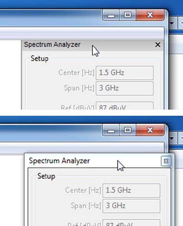
To undock any windows move the mouse pointer over the upper frame of a docked window, press and hold down the left mouse button and drag the window to the desired position (see Figure 3.1). ChipScan-Scanner will rearrange the main window in order to fit everything into it,thus all other docked windows will fill out the available space automatically. Using the undock option can bevery helpful to gain more space for the visualization on small monitors.
Additionally you can hide any docked or undocked windows by pressing the x symbol in the upper window frame. This option is especially useful if for example you evaluate your measured traces. During this task you would not need the spectrum analyzer manager at all. To show any hidden dock windows you need to select the appropriate entry from the Window menu.
You can also dock all undocked windows but the log window back to the main window. Be aware that the possible dock position varies from window to window. The spectrum analyzer manager can only be docked to the right side and the trace manager can only be docked to the bottom of the main window. To do so move the mouse pointer over the upper frame of the undocked window, press and hold down the left mouse button and drag the window over the main window. If the window oats over an allowed dock position, the window's resulting position will be automatically indicated with a shaded area.
3.1. Main menu
The main menu consists of a number of drop down menus containing speciffc important functions. The File menu contains all actions regarding ffles, the View menu holds all actions to manipulate the visualization, the Devices menu incorporates actions to manage devices, the Settings menu includes actions for spectrum analyzer settings and the Window menu contains actions to manage the dock windows. In the following all menus and their functions are listed.
| File menu | |
|---|---|
| New | Discards all traces and creates an empty file |
| Open... | Discards all traces and loads traces from a specified file |
| Save... | Saves traces to the currently opened file |
| Save as... | Saves traces and scans to a speciffed ffle |
| Import... | Appends scans in a speciffed ffle to the current scans |
| Export Scan Image... | Saves an image generated from the scan visualization to a speciffed ffle |
| Export Traces Image... | Saves an image generated from the traces visualization to a speciffed ffle |
| Export data... | Saves all traces of visualized scan as comma separated value list to a speciffed ffle |
| Exit | Closes ChipScan-Scanner |
| View menu | |
|---|---|
| Scan | Shows scan visualization only |
| Traces | Shows trace visualization only |
| Split | Shows both scan and trace visualization |
| Background color... | Sets the background color in the visualization |
| Logarithmic | Show logarithmic level values |
| Linear | Show linear level values |
| Devices menu | |
|---|---|
| Load last Setup... | Scans for recently used devices |
| Show Device Manager | Opens the device manager |
| Show Video View | Opens the video dialog |
| Hardcopy... | Generates a hard copy from the currently used spectrum analyzer and saves it to a specified file |
| Settings menu | |
|---|---|
| Scanner... | Opens scanner configuration |
| Spectrum Analyzer | |
| Center/Span | Uses center and span to set frequency range |
| Start/Stop | Uses start and stop frequency to set frequency range |
| Auto Set | Transfers settings to spectrum analyzer before any measure or take |
| Auto Save | Saves all traces to current opened ffle whenever a trace is measured |
| Absolute Measurement | Acquires an absolute measurement during take or measure |
| Relative Measurement | Acquires a relative measurement during take or measure |
| dB/Division | Sets the dB per division of the spectrum analyzer |
| Preset | Resets all settings of the spectrum analyzer to their defaults |
| Load Settings... | Loads previous saved spectrum analyzer settings from a specified file |
| Save Settings... | Saves current spectrum analyzer settings to a specified file |
| Unit | Sets the level unit of the spectrum analyzer to either dBm or dBµV |
| Window menu | |
|---|---|
| Data Set Manager | Shows the data set manager |
| Device Control | Shows the device control |
| Log | Shows the log |
| Scan Manager | Shows the scan manager |
| Trace Manager | Shows the trace manager |
| Help menu | |
|---|---|
| About... | Shows an about dialog |
| Manual... | Opens the ChipScan-Scanner manual |
3.2. Visualization
The visualization consists of two main parts. One part allows the evaluation and comparison of emission scans and the other enables you to further analyze single traces of these scans.
3.2.1. Emission scans
Due to geometry reasons the display of emission scans itself is separated into two independent visualizations; the surface/volume scan visualization and the pin/stripline scan visualization. While surface and volume scans span a 2- or 3-dimensional grid of measurement points, pin and stripline scans consists of points measured along an 1-dimensional line.
Surface and volume scans
For a speciffc frequency within the acquired frequency range all measured points are shown in a Cartesian grid (see Figure 3.2). The x-, y-, z-location of every point matches thescanner's position during measurement. Each point has a speciffc color that maps to a corresponding level value in the color bar on the right. You can switch between the acquired frequencies by moving the slider or entering a frequency value in the input ffeld below the visualization.
You are not limited to display only one frequency. You can also generate a plot for freely deffnable frequency bands. So each measurement point displays the highest level value within the band, which is really helpful to analyze multi frequency EMC problems. To enable this mode you need to check the Max Value box below the visualization, afterwards you can specify the lower and the upper frequency of the frequency band.
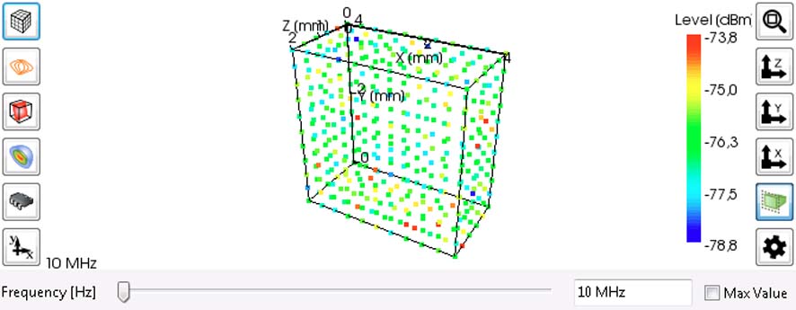
In addition to these features you can add multiple visual properties. The visibility of these properties is controlled by the buttons on the right next to the visualization.
Points ( ): Show or hide each measurement point of the emission scan.
Contour plane ( ): Show or hide a freely positionable cut plane displaying contours.
Color plane ( ): Show or hide a freely positionable cut plane displaying colors.
Isosurface( ): Show or hide isosurfaces.
Image ( ): Show or hide image of DUT.
Maximum intensity projection ( ): Project volume to x-y plane.
All properties make the qualitative analysis of EMC problems quick and easy especially for volume scans. For your convenience you can alter the size, number and opacity of the points, contours, isosurfaces and the DUT image using the properties dialog by pressing the button.
Furthermore, the visualization allows you to manipulate the view of all traces using your mouse. In the following all available mouse interactions will be explained in detail.
Navigation: To rotate the emission scan in any direction around the center of the scenemove the mouse while holding down the left mouse key over the visualization. You may additionally hold down the Ctrl key to rotate the scan around the projection axis only. Holding down the Shift key instead will move the scan along the projection plane. You can zoom in/out of the scan by spinning the scroll wheel and you can recover the full view range of the scan by pressing the button on the right next to the visualization. For your convenience you can align the view along a speciffc axis using the  ,
,  or
or  button. To switch between parallel and perspective view projection press the
  button.
Single trace analysis: When moving the mouse pointer over a speciffc measurementpoint of the emission scan a tool tip will appear showing the points' position and level. Furthermore, you will see the speciffc trace of this point in the trace visualization. To add any trace permanently do a right mouse click on the appropriate measurement point and select Add To Trace Visualization from the subsequent context menu. In this way you can easily compare the trace of any points of the emission scan against one another and even against a separate reference.
In addition the mouse context menu includes two other entries; LOCAL MAXIMUM and Global MAXIMUM To search the trace's maximum level and switch the visualization to the appropriate frequency select Local MAXIMUM If you want to search all traces of the scan for the maximum level and switch to the corresponding frequency select GlOBAL MAXIMUM When using the afore mentioned MAX VALUE mode the search of the particular maximum level is limited to the speciffed frequency band.
Pin and stripline scans
Each trace of the measured points is displayed perpendicular to the 1-dimensional line of measurement (see Figure 3.3). On the x- and the y-axis the frequency and the level is shown for a speciffc trace. The z-axis shows the trace's location according to the position on the 1-dimensional line of measurement. In addition to this data representation you may also generate a wireframe graphic connecting all traces next to each other by pressing the  button. To generate a solid surface representation press the
  button and to switch back to the normal representation use the
  button.
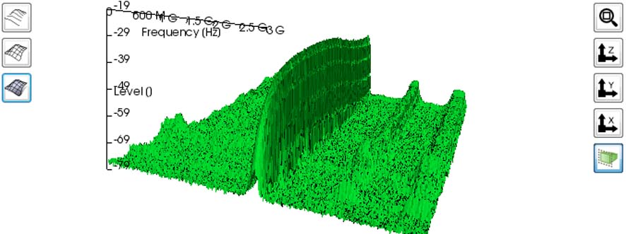
Furthermore, the visualization allows you to manipulate the view of all traces using your mouse. In the following all available mouse interactions will be explained in detail. To rotate the emission scan in any direction around the center of the scene move the mouse while holding down the left mouse key over the visualization. You may additionally hold down the Ctrl key to rotate the scan around the projection axis only. Holding down the Shift key instead will move the scan along the projection plane. You can zoom in/out of the scan by spinning the scroll wheel. Holding down the Shift key or the Ctrl key while zooming will zoom the x- or y-axis only. To recover the full view range of the scan press the button on the right next to the visualization. For your convenience you can align the view along a speciffc axis using the , or button. To switch between parallel and perspective view projection press the button.
When moving the mouse pointer over a speciffc trace of the emission scan a tool tip will appear showing the points' frequency and level. Furthermore, you will see the trace in the trace visualization. To add any trace permanently do a right mouse click on it and select Add To Trace Visualization from the subsequent context menu. In this way you can easily compare the traces of the emission scan against one another and even against a separate reference.
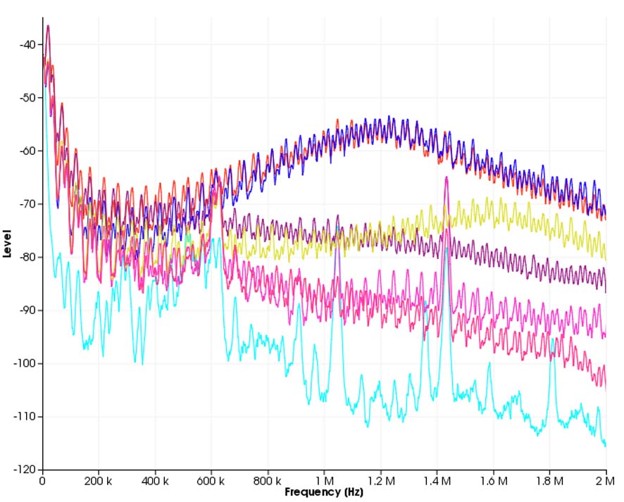
3.2.2. Single traces
All traces and corrections currently activated in the trace manager are displayed in a Cartesian coordinate system in the lower part of the visualization (see Figure 3.4). In addition it shows the trace of any emission scan point currently selected by the mouse pointer. While the x-axis' unit of the trace visualization is ffxed to Hz the y-axis' unit is not deffned. This enables you to display traces with differing units as well as correction factors in the same diagram, making analysis very easy. In addition to the traces you can show a legend containing the annotations of all visible traces in the diagram by pressing the  button on the right next to the trace visualization. For reasons of usability and to prevent the legend from covering the whole diagram the length of text of all annotations is limited to thirty characters. Other visualization options are to adapt the zoom to view all traces, to preserve current zoom and to switch between a linear or logarithmic representation of the x-axis. All of these options can be controlled via the buttons ,
  and log on the right side.
The visualization allows you to manipulate the view of all traces using your mouse. In the following all available mouse interactions will be explained in detail.
Navigation: All traces can be moved in all directions allowing you for example to center any points of interest for further investigation. To do so move the mouse pointeranywhere over the visualization, press and hold down the left mouse button, and move your mouse. While doing this the tic marks of the diagram will be updated automatically. Furthermore you can mark any trace points by pressing and holding down the right mouse button, and moving your mouse. Immediately a rectangle will be spanned to indicate a selection frame. If you release the right mouse button all trace points within the frame will be selected. This is very useful to keep track of important points when navigating or zooming within the diagram.
Zooming: To zoom in or out within the diagram you just need to spin your mouse wheel forwards or backwards. If your mouse is lacking a wheel you can alternatively press and hold down the middle mouse button, and move your mouse up or down. For reasons of convenience you can hold down the Shift or the Ctrl key while spinning the scroll wheel to zoom the diagram along the x- or the y-axis only. To recover the full view range of all visible traces press the button on the right side. Using zoom in combination with moving traces you can analyze all interesting trace points in detail.
Trace analysis: When moving your mouse pointer over any trace point a tool tip will appear at the pointer showing the measured value including the units of the data point. This enables you to exactly determine the outcome of your countermeasures regarding a speciffc EMC problem. Please keep in mind that this tool tip information is not shown, if you point the mouse on a line between two trace points.
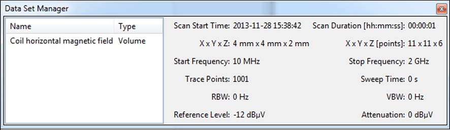
3.3. Data set manager
The data set manager lists name and type of all loaded emission scans and shows additional information like acquisition time and geometry of the currently displayed scan (see Figure 3.5). You can switch the visualization to show any emission scan by selecting the appropriate entry from the list on the left side of the data set manager. This will automatically update the emission scan information on the right side. You can also rename or delete an emission scan by right clicking on it and selecting the Rename or Delete entry from the context menu.
For further trace analysis the context menu includes a Copy to single traces entry which allows you to copy all traces of the selected emission scan to the trace visualization. We do not recommend to copy more than 1,000 traces to the trace visualization. Depending on the performance of your GPU, ChipScan-Scanner might slow down a lot rendering it unusable. In addition you can also create a maximum trace by activating the Generate maximum trace entry in the context menu. This trace holds the level maxima of all traces of the emission scan.
For your convenience the context menu also includes an option to subtract a reference scan from any surface or volume scan. The only limitation to this option is that both scans need to have the same geometry and their traces must have identical frequencies. By choosing Subtract Reference... from the context menu you can select a compatible reference scan from the subsequent dialog. This reference will be subtracted from the currently selected scan and the scan visualization will be updated automatically.
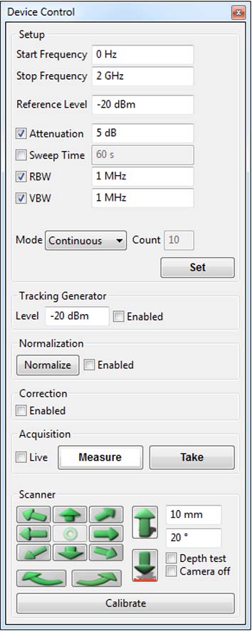
3.4. Device control
The device control (see Figure 3.6) lets you initialize and control both a connected spectrum analyzer and a Langer IC-Scanner.
3.4.1. Spectrum analyzer setup
Before setting up a spectrum analyzer make sure you properly connected it to your PC and have it identified using the device manager.2 In the following all properties are explained in detail. Keep in mind that none of the properties are transfered to your spectrum analyzer unless you press the Set button. Additionally, changes to properties done via the user interface of the spectrum analyzer are not transfered to ChipScan-Scanner. Therefore assume that the properties in the ChipScan-Scanner user interface and in the spectrum analyzer maybe out of sync.
Frequency range: You can define the frequency range of measured traces by setting a center frequency and a span. Alternatively you can also define the range using a start and a stop frequency. To switch to this mode you need to select Start/Stop from the Spectrum Analyzer sub menu in the Settings menu.
Reference level:You can set the reference level of the spectrum analyzer. The level can be defined either in dBm or in dBµV. To switch between the units use the Unit entry in the Settings menu.
Attenuation: You can either manually set the attenuation of your spectrum analyzer in dB or let the spectrum analyzer set it automatically. The latter is achieved by unchecking the box of the Attenuation field.
Sweep time: You can either manually set the sweep time of your spectrum analyzer in seconds or let the spectrum analyzer set it automatically. The latter is achieved by uncheckingthe box of the Sweep Time field.
Resolution bandwidth: You can either manually set the resolution bandwidth of your spectrum analyzer in Hz or let the spectrum analyzer set it automatically. The latter is achieved by unchecking the box of the Res. Bandw. field.
Video bandwidth: You can either manually set the video bandwidth of your spectrum analyzer in Hz or let the spectrum analyzer set it automatically. The latter is achieved by unchecking the box of the Vid. Bandw. field.
Mode: You can switch between the following modes of your spectrum analyzer; Continuous, Single, Average, Minimum Hold and Maximum Hold. If you selected the Average mode you must also define the number of traces to use to generate the average. Please see the manual of your spectrum analyzer for any details about these modes.
If you have finished to set all properties you must press the Set button to finally transfer the properties to your spectrum analyzer. Furthermore you can set the dB per division value of your spectrum analyzer using the dB/Division entry in the Spectrum Analyzer sub menu of the Settings menu. To reset your spectrum analyzer to the default settings use the Preset entry in the very same menu.
For reasons of convenience you can also store all properties for future use in a file. To do this use the Save Settings... and Load Settings... entries in the Spectrum Analyzer sub menu from the Settings menu. After loading old properties make sure to press the Set button to transfer them to your spectrum analyzer.
3.4.2. Spectrum analyzer normalization
Additionally to setting properties ChipScan-Scanner enables you to normalize your spectrum analyzer. This option is only available if your spectrum analyzer includes a supported tracking generator.
To normalize your spectrum analyzer you first need to set the output level of the tracking generator using the appropriate input field. The output level can be defined either in dBm or in dBµV. To switch between the units use the Unit entry in the Settings menu. The second step is to enable the tracking generator by enabling the box to the right of the input field. The last step is to press the Normalize button. Doing this the spectrum analyzer will generate a normalization that is applied to all following measurements. You can also enable or disable the normalization by checking or unchecking the box to the right of the Normalize button.
3.4.3. Single trace acquisition and processing
To acquire traces from your spectrum analyzer ChipScan-Scanner provides two buttons, Take and Measure. When pressing Take ChipScan-Scanner just transfers and displays the trace which is currently located in the spectrum analyzer's memory. When pressing Measure ChipScan-Scanner initiates a new measurement in the spectrum analyzer and the resulting trace is displayed in the visualization.
Additionally ChipScan-Scanner includes a LiveTrace feature. This will continuously transfer the trace from the spectrum analyzer's memory and display it together with all previously acquired traces. You can enable this feature by checking the box to the left of the Take button.
The trace processing in ChipScan-Scanner is split into three separate parts. Each of it can be controlled independently.
- Normalization of spectrum analyzer
- Application of correction factors
- Application of mathematical operators
The normalization allows a preprocessing of traces directly within the spectrum analyzer. The application of correction factors is the first step in the post-processing pipeline. In this step all correction factors enabled via the trace manager will be applied automatically to any acquired traces. You can turn on or off the application of all corrections by enabling or disabling the box under the Normalization button. The second step in the post-processing pipeline is the manual application of mathematical operators via the trace manager. Please have a look at section 3.5 for all details.
3.4.4. Scanner movement
Before initializing and moving the scanner around make sure it is properly connected to your PC and have it identified using the device manager. On successful detection you need to start the calibration of the scanner.
| Attention: Any of the following steps for scanner control may cause damage to any equipment and serious injuries or death to persons within the motion range of the scanner. Please proceed with caution while keeping all safety measures. |
To calibrate your IC-Scanner press the Calibrate button in the scanner section of the device control. This will initialize the scanner and move all axes to their zero-point position. On success you can move the scanner around by setting the drive distance and the rotation angle in the appropriate input fields. Afterwards you can use any of the arrow buttons to change the scanners relative position. While the block of nine buttons is for horizontal movement5, the two buttons right next to the block control the vertical movement and the two buttons below the block control the rotation of the probe.
In case your Langer IC-Scanner has an integrated depth test, you can activate the Depth Test box right next to the Calibrate button. If the scanner is moved downwards the integrated depth test continuously checks for a collision and therefore prevents any probe crash. In this mode the scanner moves a little slower downwards due to decelerate reasons in case of collision.
Additionally you can switch off/on the video camera directly connected to the scanner by checking/unchecking the Camera Off box.
3.4.5. Video device usage
Before using the video device connected to the scanner make sure it is detected via the device manager. To view the current stream of the video device open the video view dialog (see Figure 3.7) by selecting the Show Video entry from the Devices menu.
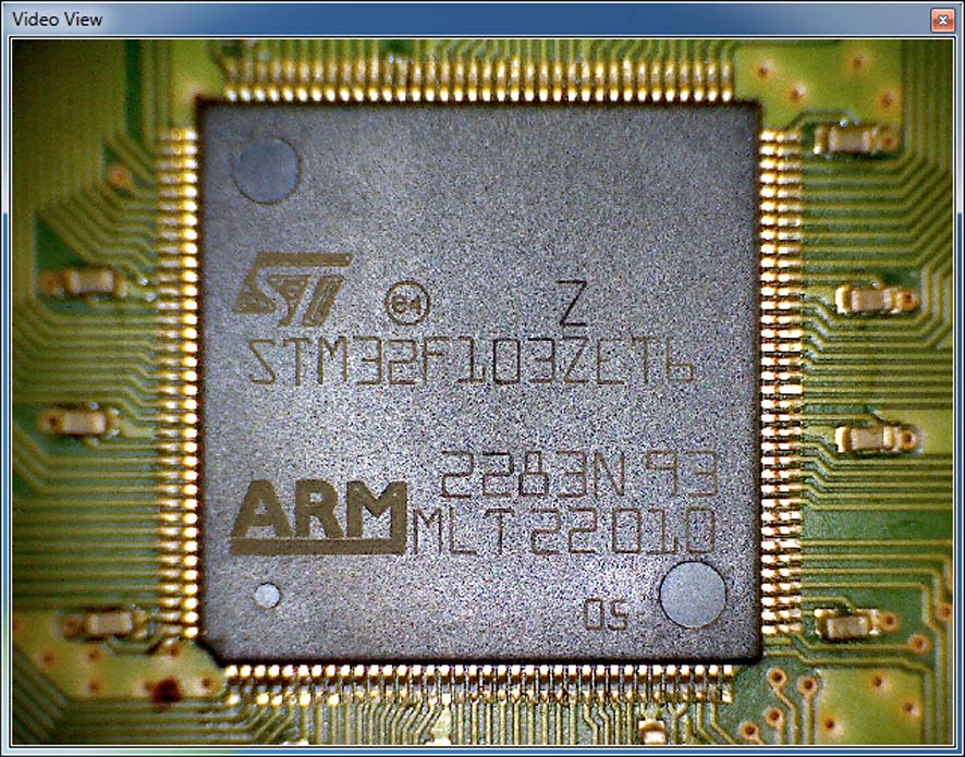
The video view allows you to manipulate the video by right clicking on it and selecting multiple options from the subsequent context menu. You can rotate the video by either 90°, 180° or 270°. You can ip it horizontal or vertical and you can switch between a low and a high resolution mode. To zoom in or out of the video view you just need to spin your mouse wheel forwards or backwards.
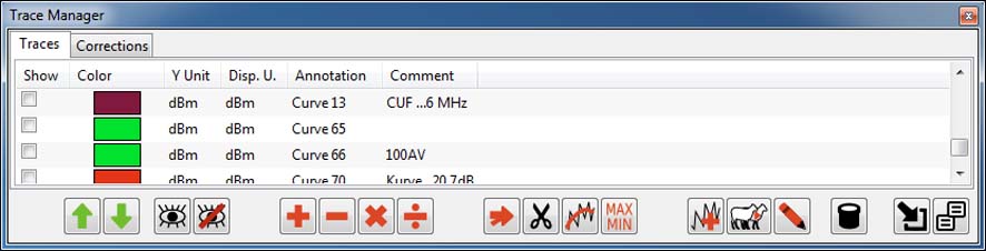
3.5. Trace manager
The trace manager holds a list of all available single traces including corrections and shows their properties; visibility, color, x- and y-axis unit, annotation and comments (see Figure 3.8). Furthermore the trace manager provides all sorts of actions to manipulate spectrum analyzer traces. You can either alter the properties of a trace or you can change the data of a trace itself. To show the trace manager press Ctrl+T or select the Trace Manager entry from the Window menu.
3.5.1. Manipulation of trace properties
Visibility: You can alter the visibility of traces in the visualization by selecting or deselecting the box in the Show column of the appropriate line in the trace manager. To show or hide multiple traces you need to select these traces in the trace manager and press  .
.
Apply: If you acquired specific correction factors for your measuring setup or you loaded special correction factors of Langer near field probes you can define their application within the measurement process. By checking or unchecking the box in the Correction column the appropriate correction will be activated or deactivated.
Color: You can change the color of a trace in the trace visualization by moving the mouse pointer over the appropriate colored rectangle in the Color column and pressing the left mouse button. In the subsequent color dialog select a new color and close the dialog.
Annotation and comment: To edit the annotation or the comment of a trace first select the appropriate line in the trace manager. Afterwards move the mouse pointer over the annotation or comment column and press the left mouse button. Now you can edit the highlighted string. Please keep in mind that the legend in the trace visualization displays only the first thirty characters of the annotation.
3.5.2. Manipulation of trace data
All actions to manipulate trace data are accomplished by pressing one of the buttons on the bottom of the trace manager. In the following the actions and the appropriate button icons are presented.
Addition, subtraction, multiplication, division (


 ): Any of these operators can be applied to a number of selected traces. For example if you press you can choose between three possibilities. You can add a constant to all selected plots, sum up all plots or add one of the selected plots to all other selected plots. Depending on your selection one or more new plots are generated and are appended to the end of the list of traces.
Merge ( ): The merge operator will merge all of the selected traces into one trace. For example if two traces define two different frequency ranges the resulting trace will contain the data points of both traces. It might happen that multiple traces have overlapping frequency ranges. Therefore when merging the traces an additional dialog is shown where you can define the merge order of the traces. The data points of the trace with the highest merge order will be chosen when merging overlapping frequency ranges.
Truncate ( ): You can truncate any number of data points from the start or the endof a trace by defining a new frequency range. Doing so will generate a new trace with alldata points lying within the specified frequency range.
Smooth ( ): You can smooth the data of a trace by applying a moving average filter with a specific width. Doing so will generate a new smoothed trace.
Min/Max ( ): You can create a maximum or minimum trace from any number of selected traces. Doing so will generate a trace that contains the maximal or minimal value of all traces for each data point.
Clone, delete (
 ): You can clone any number of selected plots. This will generate a copy of each of the selected plots in the trace manager. You can also delete any number of plots. This will permanently remove all selected plots from the trace manager.
New, edit (
 ): You can create a new trace and you can also edit any existing trace. When pressing the appropriate button of either of these operations a subsequent dialog enables you to manage all data points of a specific trace (see Figure 3.9). You can insert new points by providing a x- and a v-value, and you can change and delete any number of existing points. Furthermore you can convert both the x- or the v-values of a trace to a new unit, if there exists a specific conversion. You can also assign a new x- or y-unit to any trace. This will leave the values of the trace unchanged. If you finished all manipulations to data points make sure to press the Ok button to apply all changes. Pressing the Cancel button will abort the operation.

Import, transfer (
![]() ): You can import any number of corrections which are stored in special files having a .csc suffix. By pressing the button a file dialog opens where you can select a file containing corrections.
): You can import any number of corrections which are stored in special files having a .csc suffix. By pressing the button a file dialog opens where you can select a file containing corrections.
3.6. Log
The log collects all additional information on errors, warnings or other output which may occur during the run of ChipScan-Scanner. To show the log press Ctrl+L or select the Log entry from the Window menu. While log information is not important for the user to know it sometimes can be helpful to analyze device communication errors or other complex problems. So if you encounter any problems when running ChipScan-Scanner we recommend to read all information in the log before contacting our support. Doing so makes the process of identifying the source of your problem a lot easier. Sometimeswe may also ask you to send us all log information to exactly reproduce your problem and eliminate it.
4. Managing devices
All devices supported by ChipScan-Scanner are managed via the device manager. In general it enables you to detect all connected spectrum analyzers as well as the connected Langer IC-Scanner and to select one of them for your subsequent measurements.
4.1. Device detection
4.1.1. Device Interfaces
Spectrum analyzer By default only spectrum analyzers connected via GPIB will be detected automatically because it is the most common connection type. If you are using RS232 or LAN/VXI for connection you explicitly need to select the appropriate interface in the device manager to detect your spectrum analyzer. Make sure to disable any unused connection type to shorten the time required for detection.
When connecting via RS232 you can additionally provide the specific RS232 port your spectrum analyzer is connected to. This is especially useful to reduce the detection time, if your computer has lots of RS232 ports. When connecting via LAN/VXI you must provide the IP address or the appropriate hostname of your spectrum analyzer. Please study your spectrum analyzer manual to gain the required information.
IC-Scanner All of Langer IC-Scanners are controlled via RS232. So actually you do not need to change the interface settings at all. But to reduce detection time significantlyyou can select a specific RS232 port where your scanner is connected to.
Video camera The video device of your scanner is identified automatically.
If you set all interface properties please press the Detect Devices button to identifyyour devices.
4.1.2. Manual detection
In case of detection problems with a device you can also set all connection information manually. To do this for spectrum analyzers select your model from the drop down list and set all connection information regarding the interface in the fields above. For IC-Scanners you just need to select the model and specify the RS232 port. If you set all interface properties please press the Detect Devices button to identify your device.
4.1.3. Last setup
Whenever you close the device manager dialog the current device setup will be automatically stored, making it usable for future measurements. So if you open ChipScan-Scanner again you can use the last setup to detect your connected devices without setting the interface information. To do this select Load last Setup... in the Devices menu or open the device manager and press the Load last Setup... button.
4.2. Device selection for measurement
If the detection of devices was successful they will be added to drop down lists in the lower part of the device manager. When only one device is found it will be used automatically for the next measurements. When for example multiple spectrum analyzers are found you need to select one of them to be used for subsequent measurements. Keep in mind that you can always switch between multiple devices during your measurements.
4.3. Identifying device communication problems
All drivers for the different supported devices in ChipScan-Scanner are intensively tested. If you encounter any problems regarding your device please contact us by writing to software@langer-emv.de. But before contacting us make sure to read the following lines carefully. This may solve your problem right away.
If unable to detect a device When your device can not be detected by ChipScan-Scanner first make sure it is included in the list of supported devices (see appendix A). Then check if it is properly connected to the computer. If this is the case please use any software provided by the device manufacturer to make sure the connection between the device and your computer works. If this connection test was successful please deactivate (close) all software that might interfere with the communication between ChipScan-Scanner and your device. Especially device manufacturer software for device control or software for logging the communication over the interface are sources for errors. You may also try to perform a manual detection of your device using the device manager.
On errors during measurement If the error only occurs once please repeat your measurement. If the error occurs sporadically or continuously please deactivate (close) all software that might interfere with the communication between ChipScan-Scanner and your device. If the error persists please close and reopen ChipScan-Scanner. It might also help to restart your computer.
5. Acquisition and management of emission scans
ChipScan-Scanner allows the quick configuration and reliable execution of surface and volume emission scans using one of Langer's IC-Scanners. To acquire new emission scans or view the results of former scans open the scan manager by selecting the Scan Manager entry from the Window menu.
5.1. Scan setups
Before you can execute an emission scan a setup has to be created. The setup contains amongst general scan information, the dimension of volume to scan and the actions to perform during the scan. All the information will be included in a scan report which is created after a scan is finished. Once you created a setup you can reuse it at later time to perform the scan again with identical properties.
Before going on it might be useful to specify the path where to store the setups and the appropriate emission scan data. You can always change the path by selecting Set Data Directory entry from the Settings menu.
You can create, edit, copy and rename setups by using the appropriate buttons on the right side of the scan manager user interface (see Figure 5.1).
Creating a new setup or edit an existing setup will open a subsequent dialog (see Figure 5.2) where you can alter the specific properties of an emission scan. The different properties of an emission scan are categorized by the following tabs.
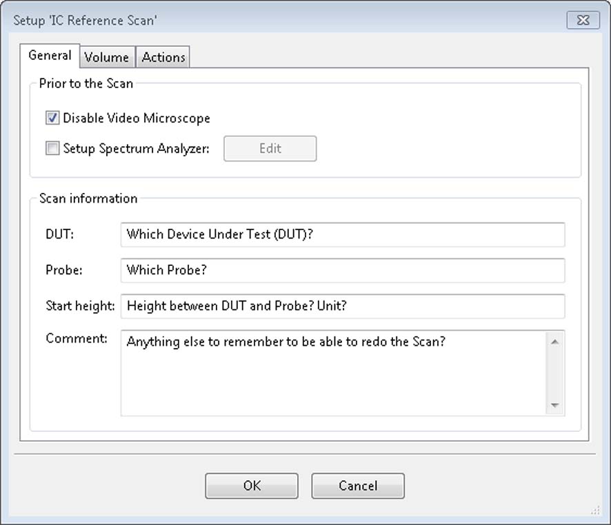
5.1.1. General properties
The general tab enables you to describe all general properties of the emission scan setup like DUT's name, the probe's name and so on. In addition you can specify to switch off the video microscope before starting the scan by checking the appropriate box in the general tab. This is especially useful to further reduce the noise level during an emission scan. You can also specify common spectrum analyzer properties, which are set in the device every time you start a scan. This enables you to repeat a scan with the exact same spectrum analyzer properties at any time. To do so check the Setup Spectrum Analyzer box and set the properties in the subsequent dialog.
5.1.2. Volume properties
For each emission scan setup the volumetric grid needs to be described. The grid is given by the x,y,z-dimension of the scan volume and the distance between two consecutive points for each axis, where the x-axis corresponds to left-right movement, the y-axis to forth-back movement and the z-axis to bottom-top movement. Keep in mind, if one of the dimensions of the volume is not divisible by its corresponding point-to-point distance, there will be a margin in this direction which is not scanned. The effective x,y,z-dimension of the scan volume, resulting by this restriction, is given below in the line Scan Volume.
5.1.3. Actions
When the scanner reaches a point on the volumetric grid, it will execute a list of actions which you can specify in the Actions tab. You can create as many actions as you want. For example you can rotate a near field probe several times at one point and measure a trace at each angle.
In addition an action contains the following set of sub actions which can be enabled separately and are executed in the given order.
- Rotate the probe
- Change the properties in the connected spectrum analyzer
- Wait for a specific time before executing the trace acquisition
- Acquire a trace using the connected spectrum analyzer
- Rotate the probe back
| Attention: Keep in mind that rotating the probe by more than 180 degree may damage the cable connection. Ensure to rotate only ±180 degree from the origin. The software itself ensures that the sum of all applied rotations in all actions is zero to avoid an increasing angle offset. |
5.2. Emission Scan Acquisition
| Attention: Any of the following steps for scanner control may cause damage to any equipment and serious injuries or death to persons within the motion range of the scanner. Please proceed with caution while keeping all safety measures. |
To start a new scan you need to select a specific setup and click on the Scan button. This opens a subsequent dialog (see fig. 5.3) where you can start a new scan, pause a running scan or abort a running scan.
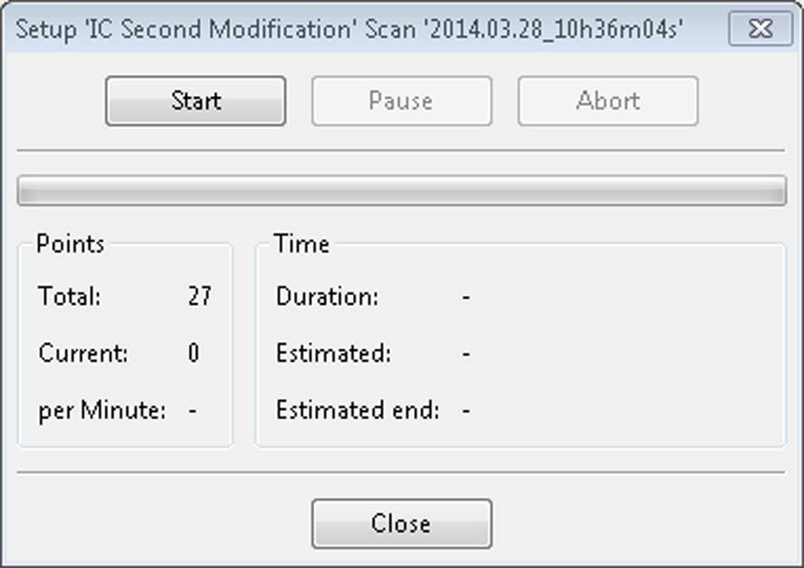
Whenever you pause or abort a scan you can always resume it in the scan manager user interface by selecting the scan from the setup tree2 and pressing the Resume button (see Figure 5.1).
To finally start a scan just hit the Start button. The scan dialog automatically updates the progress information of your emission scan.
5.3. After emission scan acquisition
At the end of each emission scan a scan report is automatically generated. To view the report press the Report button in the scan manager. The report will be opened in your default web browser and shows a maximum intensity projection of the emission scan among all other information provided in the scan setup.
If the acquisition is finished use ChipScan-Scanner to do your analysis on the scanned data. In addition you can open older scans by selecting any scan from one of your setups and press the Open button. Be aware when opening any emission scan that all currently loaded data will be closed before.
To delete any scan or setup just select it and hit the Delete button in the scan manager interface. Be aware of the following implications.
- Deletion of a scan or setup is irreversible.
- Deleting a setup deletes all appropriate scans.
6. Remote control of the scanner
ChipScan-Scanner allows you to remotely control one of Langer's IC-Scanner via XML-RPC1 for seamless integration into your own measuring setup. This is especially useful if you use LabVIEW or other software to control all of your devices. The default port number the XML-RPC server is running on is 30000 and it is displayed in the status bar of the ChipScan-Scanner GUI. You can always set the port number to a new value by selecting the Set RPC Port entry in the Settings menu.
The XML-RPC server method parameters have the following meaning:
- axisNumber: Type int with range 0 to 3 with:
- 0 for x-axis
- 1 for y-axis
- 2 for z-axis
- 3 for r-axis (rotation)
- coordinate: Type double: Specifies the absolute coordinate to move the scanner axis to within the range of the scanner axis.
- distance: Type double: Specifies the relative distance the scanner axis shall be moved within the range of the scanner axis.
- depthtest: Type bool: If set to true enables the depthtest for the z-axis, if set to false disables it.
The XML-RPC interface of ChipScan-Scanner provides the following methods including their parameters and return types:
- Void CalibrateScanner() Calibrates the scanner by moving the x-, y- and z-axis to their calibration position. This methods needs to be called once and prior to any attempt to move the scanner. This method has no return value.
- Bool IsScannerCalibrated() Returns true if the scanner is calibrated, e.g. by calling CalibrateScanner(), else returns false.
- Double GetScannerPosition(axisNumber) Returns the scanner's current axis position for the given axisNumber.
- Double GetScannerPositionMaximum(axisNumber) Returns the scanner's axis position maximum for the given axisNumber.
- Double GetScannerPositionMinimum(axisNumber) Returns the scanner's axis position minimum for the given axisNumber.
- Bool HasScannerLimitTrigger() Returns the scanner's axis position minimum for the given axisNumber. Returns true if:
- the scanner is able to move the z-axis with depthtest enabled and
- a Langer's ICR microprobe with depthtest capability is currently connected, else returns false.
- Bool IsScannerLimitTriggered() Returns true if the micropobe triggers the depthtest at the very moment, else returns false.
- Void MoveScannerAbsolute(axisNumber, coordinate, depthtest) Moves the scanner's axis for the given axisNumber to the given absolute coordinate and enables or disables the depthtest in accordance to the given depthtest parameter during the movement. The depthtest parameter is used for the z-axis only. This method has no return value.
- Void MoveScannerRelative(axisNumber, distance, depthtest) Moves the scanner's axis for the given axisNumber the given relative distance and enables or disables the depthtest in accordance to the given depthtest parameter during the movement. The depthtest parameter is used for the z-axis only. This method has no return value. Please pay attention to the possibility of rounding errors that may sum up over a lot relative movements!
7. Frequently asked questions
7.1. Windows 7 and artifacts within the visualization
If you encounter any artifacts within the visualization and you run ChipScan-Scanner on a Windows 7 system please change your current display theme to an aero theme.
Detailed description: The following artifacts have been reported within the visualization.
- switching between full screen and windowed mode of the application causes artifacts in the traces visualization
- dragging the video view over the application causes the trace visualization to stop updating the live view
- when zooming in the visualization only parts of it will be updated
7.2. Langer ICS 105 is not detected in device manager
Due to a power loss or other failures the connection between your computer and the Langer ICS 105 might be disrupted while ChipScan-Scanner runs. Detecting the Langer ICS 105 again in ChipScan-Scanner fails also if the virtual Trinamic TMCM-6110 COM device is registered in the MS Windows' device manager. If this happens please follow the steps below to solve the problem.
- close ChipScan-Scanner
- unplug and replug the USB cable connecting the ICS 105 with your computer
- reopen ChipScan-Scanner
- detect Langer ICS 105
A. Supported spectrum analyzers
The following lists contain all spectrum analyzers supported by ChipScan-ESA, the appropriate supported interfaces (RS232, GPIB1, Ethernet), the firmware version and additional important notes regarding the specific model. If you do not find your spectrum analyzer in the list please contact our sales team for available options using the following email address mail@langer-emv.com.
We are making great efforts to develop our drivers and testing them intensively. Due to different available firmwares for specific spectrum analyzer models we can not guarantee to 100 percent that all spectrum analyzers in these lists are working without any errors. Meaning of icons are:  driver fully tested,
  driver in test phase.
| Advantest | |||||
|---|---|---|---|---|---|
| Model | RS232 | GPIB | Ethernet | Firmware | Notes |
| R3131 | | ||||
| R3131A | | ||||
| R3132 | | | |||
| R3272 | | no hardcopy | |||
| U3741 | | ||||
| U3751 | | ||||
| U3771 | | ||||
| U3772 | | ||||
| Agilent | |||||
|---|---|---|---|---|---|
| Model | RS232 | GPIB | Ethernet | Firmware | Notes |
| E4401B | | | ESA-E series | ||
| E4402B | | | ESA-E series | ||
| E4403B | | | ESA-L series | ||
| E4404B | | | A.07.05 | ESA-E series | |
| E4405B | | | ESA-E series | ||
| E4407B | | | ESA-E series | ||
| E4408B | | | ESA-L series | ||
| E4411B | | | ESA-L series | ||
| E7401A | | | A.02.00 | EMC series | |
| E7402A | | | EMC series | ||
| E7403A | | | EMC series | ||
| E7404A | | | EMC series | ||
| E7405A | | | A.14.04 | EMC series | |
| N9000A | | | A.07.06 | CXA series | |
| N9010A | | | A.14.06 | EXA series | |
| N9020A | | | A.10.52 | MXA series | |
| N9030A | | | A.07.04 | PXA series | |
| N9320B | | 0B.03.43 | no hardcopy, no preset, nouncal | ||
| Hameg | |||||
|---|---|---|---|---|---|
| Model | RS232 | GPIB | Ethernet | Firmware | Notes |
| HM5014 | | ||||
| HM5014-2 | | ||||
| HM5530 | | ||||
| Rigol | |||||
|---|---|---|---|---|---|
| Model | RS232 | GPIB | Ethernet | Firmware | Notes |
| DSA815 | | 00.01.08.00.03 | slow data aquisition | ||
| Rohde & Schwarz | |||||
|---|---|---|---|---|---|
| Model | RS232 | GPIB | Ethernet | Firmware | Notes |
| ESL3 | | 1.83 SP4 | |||
| ESL6 | | ||||
| ESPI3 | | no tracking generator yet | |||
| ESPI7 | | 4.42 | no tracking generator yet | ||
| ESR3 | | | no tracking generator yet | ||
| ESR7 | | | 2.27 SP1 | no tracking generator yet | |
| ESR26 | | | no tracking generator yet | ||
| ESRP3 | | | no tracking generator yet | ||
| ESRP7 | | | 2.26 | no tracking generator yet | |
| ESU8 | | | | 4.43 | hardcopy via GPIB only, no tracking generator yet |
| ESU26 | | | | hardcopy via GPIB only, no tracking generator yet | |
| ESU40 | | | | hardcopy via GPIB only, no tracking generator yet | |
| ETL3 | | | 1.73 | ||
| FSH3 | | several issues | |||
| FSH4 | | no tracking generator | |||
| FSH6 | | V07.11 | several issues | ||
| FSH8 | | V2.50 | no tracking generator | ||
| FSH13 | | no tracking generator | |||
| FSH18 | | several issues | |||
| FSH20 | | no tracking generator | |||
| FSL3 | | | 2.00 SP2 | ||
| FSL6 | | | 1.80 SP1 | ||
| FSL18 | | | 1.80 SP1 | ||
| FSP3 | | | |||
| FSP7 | | | 4.50 | ||
| FSP13 | | | 2.80 | ||
| FSP30 | | | |||
| FSP31 | | | |||
| FSP40 | | | |||
| FSU3 | | | no tracking generator yet | ||
| FSU8 | | | no tracking generator yet | ||
| FSU26 | | | 4.37 | no tracking generator yet | |
| FSU31 | | | no tracking generator yet | ||
| FSU32 | | | no tracking generator yet | ||
| FSU43 | | | no tracking generator yet | ||
| FSU46 | | | no tracking generator yet | ||
| FSU50 | | | no tracking generator yet | ||
| FSU67 | | | no tracking generator yet | ||
| FSUP8 | | | |||
| FSUP26 | | | 4.37 | ||
| FSUP50 | | | |||
| FSV3 | | | 1.50 | ||
| FSV7 | | | |||
| FSV13 | | | 1.50 | ||
| FSV30 | | | |||
| FSV40 | | | |||
| RTO1002 | | FFT on MATH1 channel | |||
| RTO1004 | | FFT on MATH1 channel | |||
| RTO1012 | | FFT on MATH1 channel | |||
| RTO1014 | | FFT on MATH1 channel | |||
| RTO1022 | | FFT on MATH1 channel | |||
| RTO1024 | | 2.40.1.1 | FFT on MATH1 channel | ||
| RTO1044 | | FFT on MATH1 channel | |||
| Tektronix | |||||
|---|---|---|---|---|---|
| Model | RS232 | GPIB | Ethernet | Firmware | Notes |
| RSA6106A | | | no hardcopy | ||
| RSA6114A | | | FV:2.1.0098 | no hardcopy | |
| RSA6120A | | | no hardcopy | ||
Downloads
ChipScan-Scanner 3.0.14 - Supported Spectrum Analyzers
To get a demo version of our software for free, please contact our sales team: sales@langer-emv.de